Exploring the Depths of a Pivot Table: A Step-by-Step Guide

When it comes to analyzing and presenting data, pivot tables are a powerful tool that can reveal valuable insights. While they may seem complex at first, understanding how to use a pivot table can greatly enhance your data analysis capabilities. In this step-by-step guide, we will demystify the pivot table and provide you with the knowledge and skills to confidently explore the depths of this invaluable analytical tool.
To begin, let’s define what a pivot table is. At its core, a pivot table is a data summarization tool that allows you to extract meaningful information from large datasets. By organizing and manipulating data, pivot tables provide a way to aggregate, sort, and filter information, allowing for easier analysis and visualization.
One of the key features of a pivot table is its ability to dynamically rearrange and reorganize data. With just a few clicks, you can change the layout of the table, move columns and rows, and quickly experiment with different ways of summarizing your data. This flexibility makes pivot tables incredibly versatile and adaptable to various data analysis scenarios.
Note: While pivot tables can be created in various software applications, such as Microsoft Excel and Google Sheets, the concepts and principles discussed in this guide can be applied to any pivot table implementation.
In this guide, we will explore the step-by-step process of creating a pivot table, from selecting the data source and choosing the appropriate fields, to customizing the layout and applying calculations. We will also delve into advanced features, such as filtering, grouping, and creating calculated fields, to further refine and analyze your data. By the end of this guide, you will have a solid understanding of pivot tables and the confidence to apply this valuable tool to your own data analysis projects.
What is a Pivot Table and Why Should You Use It?
A pivot table is a powerful data analysis tool that allows you to summarize and rearrange large amounts of data into a more manageable and meaningful format. It is commonly used in spreadsheets and database programs, such as Microsoft Excel or Google Sheets.

Benefits of Using a Pivot Table:
- Easy Data Analysis: Pivot tables simplify the process of analyzing large datasets by allowing you to quickly and easily summarize, sort, and filter data based on various criteria.
- Data Summarization: With a pivot table, you can summarize data by calculating sums, averages, counts, or other functions on data values. This helps you gain insights and draw conclusions from your data quickly.
- Data Rearrangement: Pivot tables allow you to rearrange and reorganize data in a way that makes it easier to understand and analyze. You can drag and drop fields to create new arrangements and instantly see the impact on the data.
- Flexible Data Filtering: Pivot tables provide powerful filtering options, allowing you to focus on specific subsets of data that meet certain criteria. This enables you to analyze different aspects of your data and answer specific questions.
Overall, the use of pivot tables can greatly enhance your data analysis capabilities and help you make informed decisions based on your data. It allows you to quickly explore different perspectives of your data and uncover valuable insights that may have otherwise gone unnoticed.
Step 1: Understanding the Structure and Layout of a Pivot Table
A pivot table is a powerful tool in spreadsheet software that allows you to summarize and analyze large sets of data. Before diving into creating a pivot table, it is important to understand its structure and layout.
1. Rows, Columns, and Values
A pivot table consists of three main areas: rows, columns, and values. These areas define how the data will be summarized and organized in the table.
- Rows: This area represents the categories or groups that you want to display on the vertical axis of the table. For example, if you are analyzing sales data, the rows could represent different products or regions.
- Columns: This area represents the categories or groups that you want to display on the horizontal axis of the table. It allows you to compare data across different categories. Using the previous example, columns could represent different months or years.
- Values: This area represents the numerical data that you want to summarize or analyze. It can be any kind of numerical data, such as sales revenue or customer count.
2. Pivot Fields

The data in a pivot table comes from a source range or table in your spreadsheet. Each column in the source data becomes a “pivot field” in the pivot table. These fields are used to populate the rows, columns, and values of the table.
- Row Labels: These are the fields that determine the rows in the pivot table. They are displayed in the rows area.
- Column Labels: These are the fields that determine the columns in the pivot table. They are displayed in the columns area.
- Values: These are the fields that provide the numerical data to be summarized or analyzed in the pivot table. They are displayed in the values area.
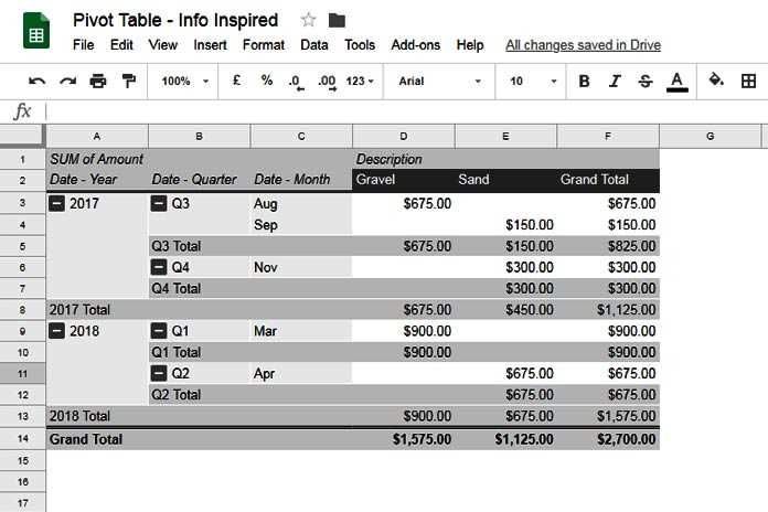
3. Subtotals and Grand Totals
A pivot table automatically calculates subtotals and grand totals for the rows and columns. Subtotals are calculated for each group within a category, while grand totals represent the totals for all data in the table.
4. Filtering, Sorting, and Formatting
Pivot tables offer various options to filter, sort, and format the data. You can filter the data to focus on specific categories or ranges, sort the data in ascending or descending order, and apply formatting to make the table more visually appealing.
5. Refreshing the Pivot Table
As the source data in your spreadsheet changes, you can refresh the pivot table to update the summary and analysis. This ensures that the pivot table always reflects the latest data.

By understanding the structure and layout of a pivot table, you can effectively set up and customize your pivot table to analyze and summarize your data in a meaningful way.
Step 2: Importing and Organizing Your Data
In order to create a pivot table, you first need to import and organize your data. This step is crucial as it determines the accuracy and effectiveness of your analysis. Follow the steps below to import and organize your data:
1. Prepare your data
Make sure your data is structured properly and contains all the necessary fields. You can use spreadsheets or databases to store your data. Ensure that each column represents a unique attribute or variable, and each row represents an individual record or data point.
2. Open a new Excel workbook
Launch Microsoft Excel and open a new workbook to begin your pivot table creation process. You can also choose to work with an existing workbook if you have data that needs to be analyzed.
3. Import your data

Import your data into Excel by navigating to the “Data” tab and selecting the desired import method. You can choose to import data from a variety of sources including spreadsheets, databases, and online sources. Follow the prompts to connect to your data source and import the desired data into Excel.
4. Organize your data
Once your data is imported, organize it in a table format to make it easier for Excel to recognize and analyze. You can do this by selecting your data range and converting it into an Excel table. To convert your data into a table, go to the “Insert” tab and click on the “Table” button. Make sure to check the box that says “My table has headers” if your data has column headers.
5. Clean and format your data
Before proceeding with creating a pivot table, it is important to clean and format your data if necessary. Remove any unnecessary rows, columns, or data points that are irrelevant to your analysis. Ensure that your data is in the correct format (i.e., numbers are formatted as numbers, dates are formatted as dates, etc.). This will help to avoid any errors or inconsistencies in your final pivot table.
6. Save your workbook
After organizing and cleaning your data, save your workbook in order to preserve your progress. This will allow you to easily access and update your data in the future.
By following these steps, you will be able to successfully import and organize your data in preparation for creating a pivot table. The next step is to actually create the pivot table itself, which will be covered in the next section of this guide.

Step 3: Choosing the Right Fields for Your Pivot Table
Now that you have selected your data source and arranged it in a structured manner, it’s time to choose the right fields for your pivot table. This step is crucial as it determines how your data will be analyzed and presented.
1. Rows
The first step is to select the fields that will be used as rows in your pivot table. These fields categorize your data and determine the structure of your table. You can choose multiple fields to create a hierarchical structure.
- Select a field: Choose a field that represents a category or grouping of your data. For example, if you have sales data, you could choose the “Region” field to group sales by different regions.
- Add more fields (optional): If you want to further categorize your data, you can add more fields as subcategories. For example, you could add the “Product” field to further segment sales by different products within each region.
2. Columns
The next step is to select the fields that will be used as columns in your pivot table. These fields provide a way to compare data across different categories or segments.
- Select a field: Choose a field that represents a specific characteristic or attribute of your data. For example, if you want to compare sales data across different years, you could choose the “Year” field as a column.
- Add more fields (optional): If you want to compare data across multiple attributes, you can add more fields as additional columns. For example, you could add the “Month” field to further segment sales by different months within each year.
3. Values
The final step is to select the fields that will be used as values in your pivot table. These fields contain the actual data that you want to summarize, analyze, or perform calculations on.

- Select a field: Choose a field that contains the data you want to analyze or summarize. For example, you could choose the “Sales” field if you want to analyze the total sales for each combination of categories.
- Add more fields (optional): If you want to perform calculations on multiple fields, you can add more fields as additional values. For example, you could add the “Profit” field to analyze the total sales and profit for each combination of categories.
By carefully choosing the right fields for your pivot table, you can gain valuable insights into your data and easily compare and analyze different aspects of your data.
Step 4: Grouping and Sorting Data within Your Pivot Table
Once your pivot table is created and the data is properly organized, you may want to group and sort the data to gain further insights. This step will guide you through the process of grouping and sorting your data within the pivot table.
Grouping Data
Grouping your data allows you to combine certain values into categories, making it easier to analyze and understand the information in your pivot table. To group data, follow these steps:
- Select the column or row that you want to group.
- Right-click within the selected area and choose the “Group” option.
- Specify the grouping criteria, such as grouping by months, quarters, or years.
- Click “OK” to apply the grouping to your pivot table.
By grouping your data, you can create a more organized and structured view of your data, allowing for better analysis and trend identification.
Sorting Data
Sorting data within a pivot table is useful when you want to arrange the values in a specific order, such as ascending or descending. To sort data, follow these steps:

- Select the column or row that you want to sort.
- Right-click within the selected area and choose the “Sort” option.
- Select the desired sorting order, such as ascending or descending.
- Click “OK” to apply the sorting to your pivot table.
Sorting data within your pivot table allows you to arrange the values in a way that makes it easier to analyze and find patterns in your data.
By grouping and sorting your data within your pivot table, you can better organize and analyze your information, making it easier to extract valuable insights and make data-driven decisions.
Step 5: Adding Calculated Fields and Formulas
In addition to summarizing data, pivot tables also allow you to create calculated fields and apply formulas to your data. This can be useful for performing calculations that are not available directly from your raw data.
Creating a Calculated Field
To create a calculated field, follow these steps:
- Select the pivot table.
- Go to the “PivotTable Analyze” or “Options” tab in the Excel ribbon (depending on your Excel version).
- Click on the “Fields, Items & Sets” drop-down button.
- Select “Calculated Field” from the drop-down menu.
- In the “Name” field, enter a name for your calculated field.
- In the “Formula” field, enter the formula for your calculated field. You can use any of the available mathematical operators (+, -, *, /) and functions like SUM, AVERAGE, COUNT, etc.
- Click on the “Add” button to create the calculated field.
Once created, the calculated field will appear as a new field in your pivot table’s field list. You can now drag and drop it into your pivot table to include the calculated values.
Applying Formulas to Pivot Data
In addition to calculated fields, you can also apply formulas directly to the values in your pivot table. This can be useful for performing calculations on subsets of your data or combining multiple fields.
To apply a formula to a pivot table, follow these steps:
- Select the cell where you want to enter the formula.
- Type an equals sign (=) to start the formula.
- Select the cell or cells that you want to include in the formula. You can use the arrow keys or the mouse to select cells within the pivot table.
- Enter the desired mathematical operators and functions to construct your formula. Remember to use parentheses to control the order of operations.
- Press Enter to apply the formula to the selected cell.
The formula will be applied to the selected cell and the result will be displayed. The formula will also be automatically updated if the underlying data in the pivot table changes.
Using calculated fields and applying formulas can enhance the analysis capabilities of your pivot table and allow you to perform more complex calculations on your data.
Summary
In Step 5, we explored the ability of pivot tables to create calculated fields and apply formulas. This enables us to perform calculations that are not available directly from the raw data. By following the steps outlined in this section, you can add calculated fields and apply formulas to your pivot table, providing more insights into your data.
Step 6: Customizing the Look and Feel of Your Pivot Table
Customizing the Appearance
Once you have created your pivot table and organized the data, you might want to customize the look and feel of your pivot table to make it more visually appealing and easily readable. There are several ways to achieve this:
- Formatting Options: You can change the font, color, alignment, and other formatting options for your pivot table. This can be done by selecting the cells or ranges you want to format and using the formatting options in the toolbar.
- Conditional Formatting: Another way to enhance the visual appeal of your pivot table is by applying conditional formatting. This allows you to highlight specific cells based on certain conditions. For example, you can make cells with values above a certain threshold appear in green, or cells with negative values appear in red.
- Themes: Pivot tables can be styled using predefined themes that change the overall appearance of the table. You can choose from a variety of built-in themes or create your own custom theme to match your preferences or the overall design of your report or presentation.
Customizing the Layout
In addition to changing the appearance, you can also customize the layout of your pivot table to improve the overall organization and readability of the data:
- Adjusting Column Widths and Row Heights: You can resize the columns and rows in your pivot table to ensure that the data is properly displayed. This can be done by clicking and dragging the column or row headers to the desired size.
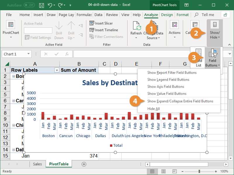
- Collapsing and Expanding Fields: If your pivot table contains multiple fields, you can collapse or expand them to hide or display the underlying data. This can be especially useful when dealing with large datasets or when you only want to focus on specific parts of the data.
- Grouping and Subtotaling: Pivot tables allow you to group data based on certain criteria, such as dates or categories. This can make it easier to analyze the data and identify trends or patterns. Additionally, you can add subtotals and grand totals to provide a summary of the data at different levels.
Summary
Customizing the look and feel, as well as the layout of your pivot table, can greatly enhance the presentation and readability of your data. By applying formatting options, conditional formatting, and themes, you can make your pivot table visually appealing and easy to understand. Additionally, adjusting the layout by resizing columns and rows, collapsing and expanding fields, and grouping and subtotaling data can help you organize and analyze your data effectively.
Step 7: Filtering and Slicing Your Pivot Table Data
Filtering Your Pivot Table
One of the most powerful features of a pivot table is the ability to filter the data based on specific criteria. Filtering allows you to focus on the information that is most relevant to your analysis. Here’s how you can filter your pivot table data:
- Click on the drop-down arrow next to the field you want to filter. This will open a list of all the unique values in that field.
- Select the specific value or values you want to include or exclude from your pivot table.
- Click OK to apply the filter.
By applying a filter, you can narrow down your data to display only the information that meets your desired criteria. This can be helpful when you want to analyze only a specific category or subset of your data.
Slicing Your Pivot Table
Another way to analyze your pivot table data is by slicing it, which allows you to break down the information based on different dimensions or hierarchies. Slicing provides a more detailed view of your data by splitting it into smaller segments. Here’s how you can slice your pivot table:
- Select the field you want to slice your data by.
- Drag and drop the field into the “Columns” or “Rows” area of your pivot table.
Once you’ve sliced your pivot table, you can easily compare and analyze the data across different categories or dimensions. This can be helpful when you want to identify trends, patterns, or relationships within your data.
Using Multiple Filters and Slicers
You can apply multiple filters and slicers to your pivot table to further refine your analysis. This allows you to drill down into your data and uncover deeper insights. Here are some tips for using multiple filters and slicers:
- To apply multiple filters, repeat the filtering process for each field you want to filter by.
- To apply multiple slicers, drag and drop the desired fields into the “Slicers” area of your pivot table. This will create separate slicer controls for each field.
- You can customize the appearance of your slicers by right-clicking on them and selecting “Slicer Settings”. Here, you can change the slicer style, layout, and other options.
By leveraging multiple filters and slicers, you can perform in-depth analyses of your pivot table data and gain a comprehensive understanding of your dataset.
Conclusion
Filtering and slicing your pivot table data are essential techniques to explore and analyze your data in a more focused and detailed manner. By applying filters and using slicers, you can extract valuable insights and make data-driven decisions. Experiment with different filtering and slicing options to uncover patterns, trends, and relationships within your data.
FAQ:
What is a pivot table?
A pivot table is a data summarization tool in spreadsheet software that allows you to quickly analyze and summarize large amounts of data.
How does a pivot table work?
A pivot table works by automatically grouping and aggregating data based on specified criteria. It allows you to organize and rearrange data to see different perspectives and patterns.
What can you do with a pivot table?
With a pivot table, you can perform tasks such as summarizing data, calculating totals and subtotals, creating custom calculations, filtering data, and creating visualizations like charts and graphs.
How do I create a pivot table?
To create a pivot table, you need to select your data range, go to the “Insert” tab, click on “PivotTable,” select your data range again, specify where you want the pivot table to be placed, and then follow the prompts to set up the pivot table fields.
Can I update my pivot table if my data changes?
Yes, you can update your pivot table if your data changes. Simply right-click on the pivot table, click on “Refresh,” and the pivot table will be updated with the latest data.
Can I customize the appearance of my pivot table?
Yes, you can customize the appearance of your pivot table by changing the layout, applying styles, formatting numbers, adding conditional formatting, and using different themes and colors.
What are some advanced features of pivot tables?
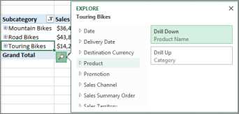
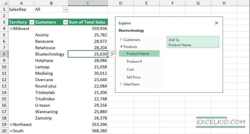
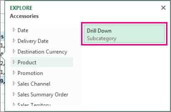
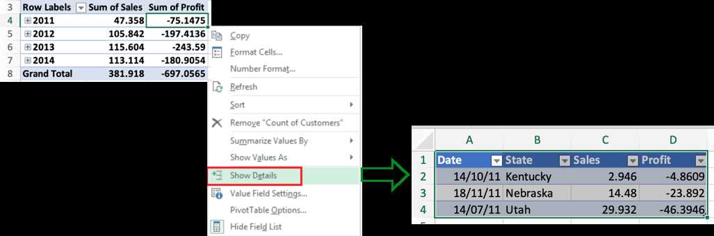
Some advanced features of pivot tables include creating calculated fields and items, sorting and filtering data, using timeline filters, adding slicers, drilling down to details, and connecting multiple data sources.
Video:


Meet Harrison Clayton, a distinguished author and home remodeling enthusiast whose expertise in the realm of renovation is second to none. With a passion for transforming houses into inviting homes, Harrison's writing at https://thehuts-eastbourne.co.uk/ brings a breath of fresh inspiration to the world of home improvement. Whether you're looking to revamp a small corner of your abode or embark on a complete home transformation, Harrison's articles provide the essential expertise and creative flair to turn your visions into reality. So, dive into the captivating world of home remodeling with Harrison Clayton and unlock the full potential of your living space with every word he writes.


